
Set-boundary based Reachability Analysis Toolbox in Python
Reachability analysis, which computes sets of states reachable by a system over time, plays a fundamental role in the temporal verification of nonlinear systems. In practice, however, overly pessimistic over-approximations often render many temporal properties unverifiable. This pessimism mainly arises from the wrapping effect, namely the propagation and accumulation of over-approximation errors during the iterative construction of reachable sets. Since the severity of the wrapping effect strongly correlates with the volume of the initial set, partitioning-based techniques—where the initial state space is divided into smaller subsets and analyzed independently—are commonly employed to mitigate this effect, especially for large initial sets and long time horizons (see here). Such partitioning, however, typically incurs substantial computational and memory overhead, often making existing reachability analysis techniques unsuitable for complex real-world applications. In particular, being forced to explore the full—often exponential in the system dimension—number of partitions severely limits scalability. Motivated by this challenge, this tool implements the so-called set-boundary–based method, which computes the full reachable state space by performing state-exploratory analysis on only a small sub-volume of the initial set, namely a set enclosing its boundary. By avoiding exhaustive exploration of the interior, this approach significantly improves scalability while preserving soundness. For theoretical foundations, please refer to Bai Xue et al., “Reach-Avoid Verification for Nonlinear Systems Based on Boundary Analysis,” IEEE Transactions on Automatic Control, 2017, and Bai Xue et al., “Over- and Under-Approximating Reach Sets for Perturbed Delay Differential Equations,” IEEE Transactions on Automatic Control, 2020.
The set-boundary–based method can be used to perform reachability analysis for systems modeled by:
- Ordinary differential equations (ODEs) with Lipschitz-continuous perturbations,
- Delay differential equations (DDEs) with Lipschitz-continuous perturbations,
- Neural ordinary differential equations (Neural ODEs).
PyBDR requires Python 3.11 or newer and runs on Linux, macOS and Windows. All dependencies are regular Python packages, no system library has to be installed.
pip install "pybdr @ git+https://github.com/ASAG-ISCAS/PyBDR"Optional extras:
pybdr[vis]adds plotly for interactive 3D plots.pybdr[test]adds pytest to run the test suite.
To work on PyBDR, install it in editable mode with the development tools, in a virtual environment with Python 3.11 or newer:
git clone https://github.com/ASAG-ISCAS/PyBDR.git
cd PyBDR
pip install -e ".[dev]"
pytest -m "not slow"        # the slow tests execute the example notebooks
Before a commit, python scripts/run_checks.py runs the tests and all example notebooks and writes a
report to reports/summary.md (see examples/).
Open the demo notebook in Colab with the button below, its first cell installs PyBDR. It verifies whether a car changing lanes can hit obstacles, starting from a non-convex set of initial states. examples/ has a notebook for every algorithm, stored with its results so that they can be viewed on GitHub directly.

The tool provides sample files which serve as demonstrations of the proper utilization for computing reachable sets. These sample files serve as a reference point for users to grasp the process of modifying the dynamics and parameters necessary for reachability analysis. This feature aids users in experimenting with their analyses, allowing them to assess the impact of different settings on the overall computation of the reachable sets
For example, consider the following dynamic system:
import numpy as np
from pybdr.algorithm import ASB2008CDC
from pybdr.util.functional import performance_counter, performance_counter_start
from pybdr.geometry import Zonotope, Interval, Geometry
from pybdr.geometry.operation import boundary, cvt2
from pybdr.model import *
from pybdr.util.visualization import plot

# reach_parallel starts worker processes, which requires this guard on macOS and Windows
if __name__ == "__main__":
    # settings for the computation
    options = ASB2008CDC.Options()
    options.t_end = 6.74
    options.step = 0.005
    options.tensor_order = 3
    options.taylor_terms = 4
    options.u = Zonotope.zero(1, 1)
    options.u_trans = np.zeros(1)

    # settings for the using geometry
    Zonotope.REDUCE_METHOD = Zonotope.REDUCE_METHOD.GIRARD
    Zonotope.ORDER = 50

    z = Interval([1.23, 2.34], [1.57, 2.46])
    x0 = cvt2(z, Geometry.TYPE.ZONOTOPE)
    xs = boundary(z, 1, Geometry.TYPE.ZONOTOPE)

    this_time = performance_counter_start()
    ri_without_bound, rp_without_bound = ASB2008CDC.reach(vanderpol, [2, 1], options, x0)
    this_time = performance_counter(this_time, 'reach_without_bound')

    ri_with_bound, rp_with_bound = ASB2008CDC.reach_parallel(vanderpol, [2, 1], options, xs)
    this_time = performance_counter(this_time, 'reach_with_bound')

    # visualize the results
    plot(ri_without_bound, [0, 1])
plot(ri_with_bound, [0, 1])| With Boundary Analysis (BA) | No Boundary Analysis (NBA) |
|---|---|
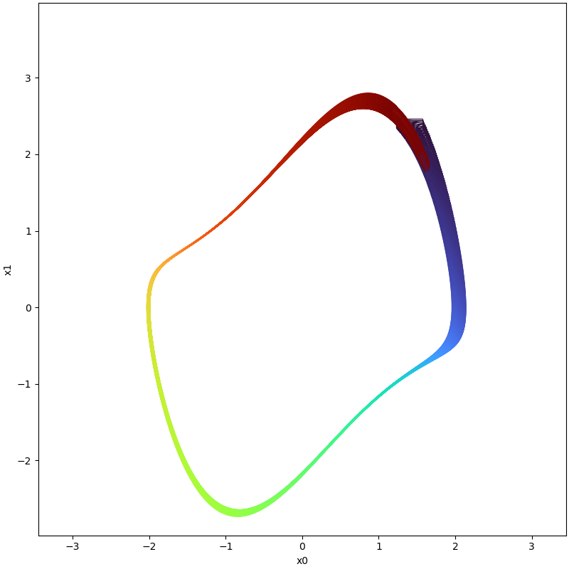 |
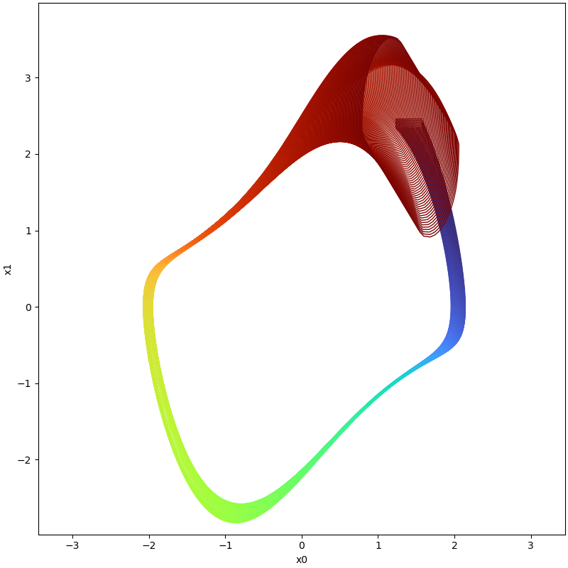 |
For large initial sets,
| System | Code | Reachable Sets (Orange-NBA,Blue-BA) |
|---|---|---|
| synchronous machine | benchmark_synchronous_machine_cmp.py | 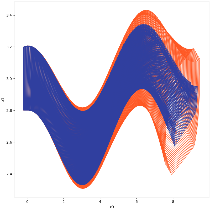 |
| Lotka Volterra model of 2 variables | benchmark_lotka_volterra_2d_cmp.py | 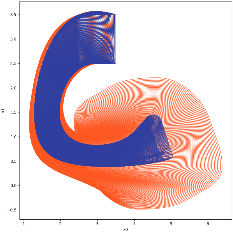 |
| Jet engine | benchmark_jet_engine_cmp.py | 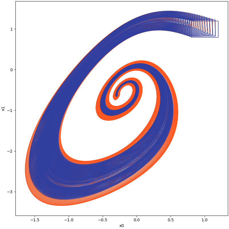 |
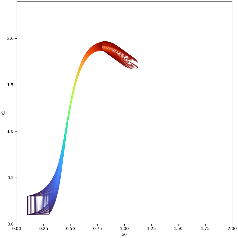
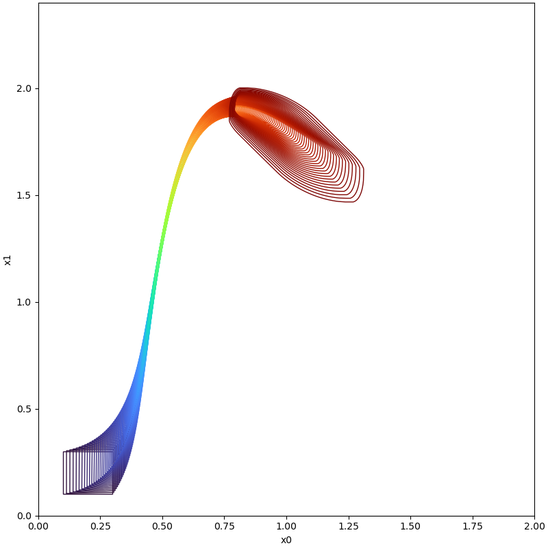
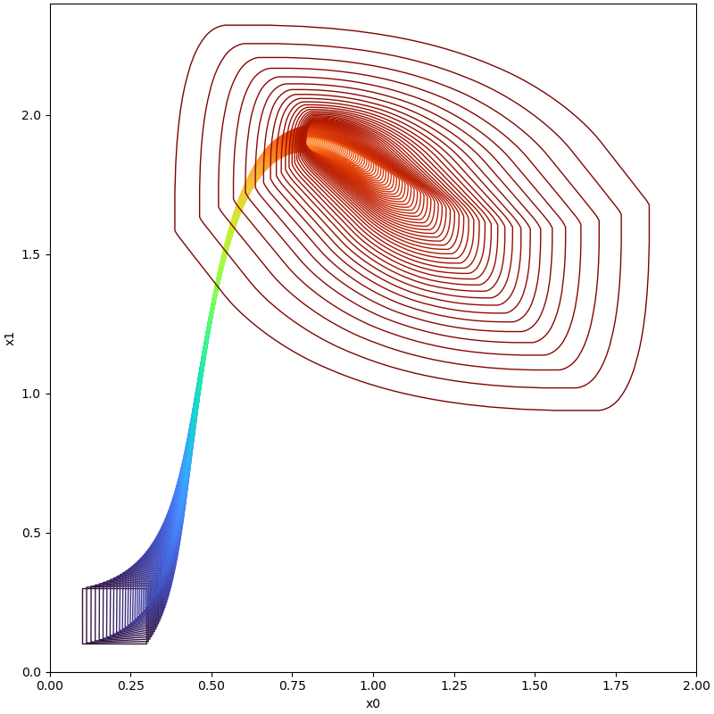
For large time horizons, i.e. consider the system Brusselator
For more details about the following example, please refer to our code.
| Time instance | With Boundary Analysis | Without Boundary Analysi |
|---|---|---|
| t=5.4 | 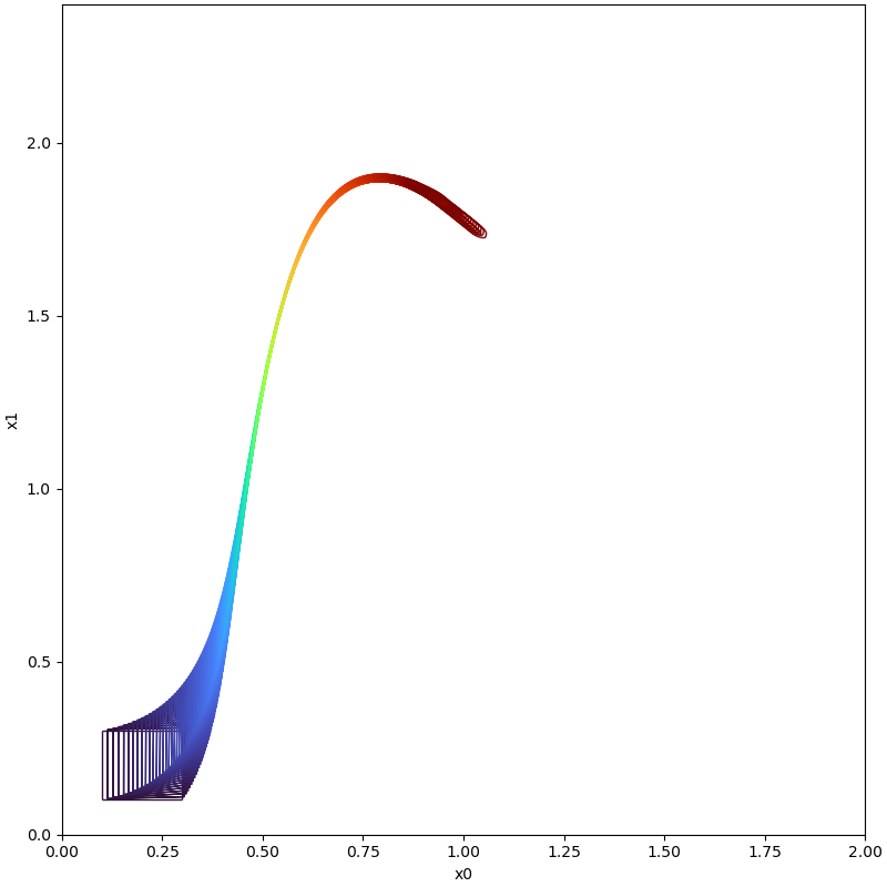 |
 |
| t=5.7 | 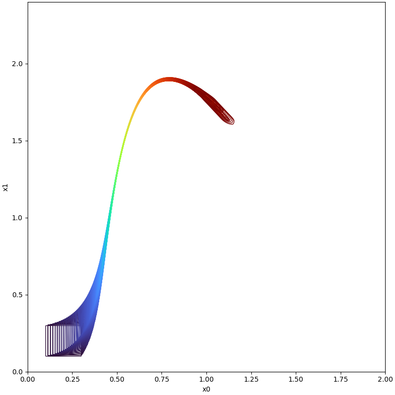 |
 |
| t=6.0 | 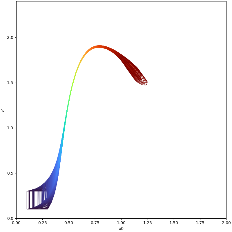 |
 |
| t=6.1 | 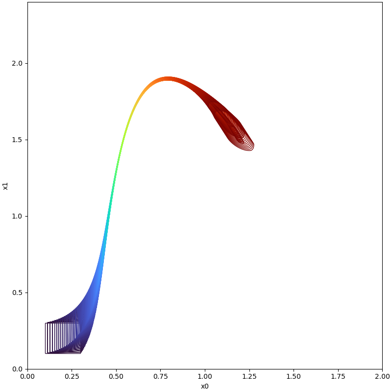 |
Set Explosion Occurred! |
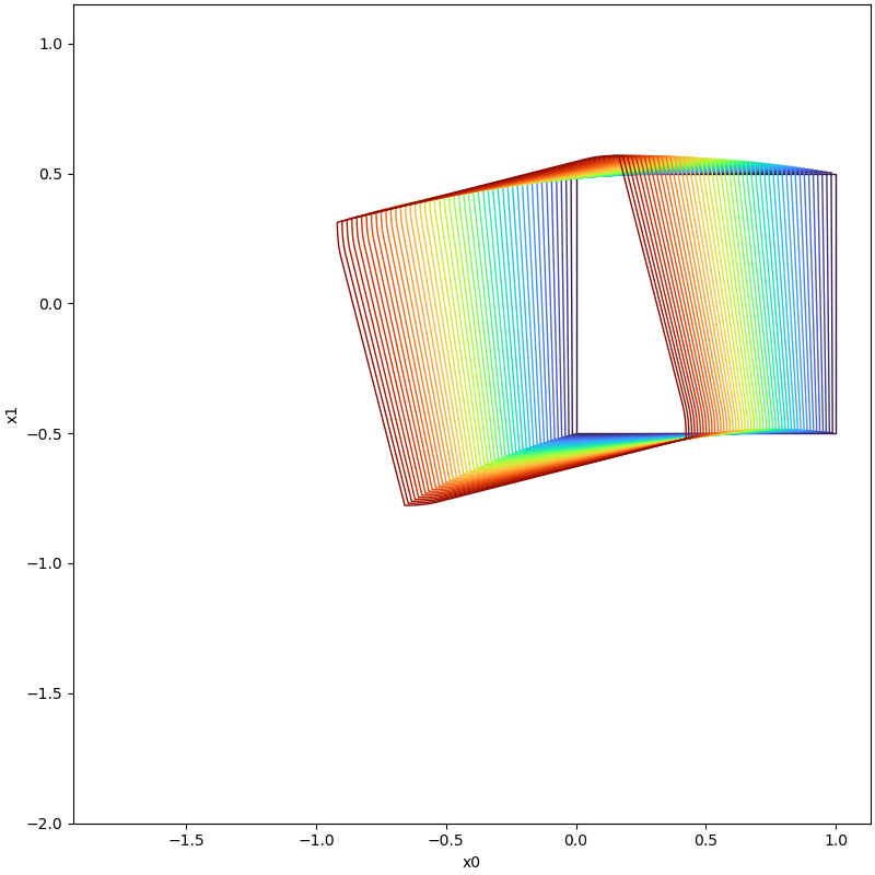
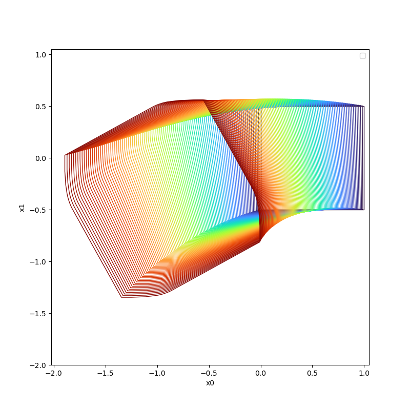
For example, consider a neural ODE with the following parameters and
import numpy as np

from pybdr.algorithm import ASB2008CDC
from pybdr.geometry import Zonotope, Interval, Geometry
from pybdr.model import *
from pybdr.util.visualization import plot, plot_cmp
from pybdr.geometry.operation import boundary, cvt2
from pybdr.util.functional import performance_counter_start, performance_counter

# reach_parallel starts worker processes, which requires this guard on macOS and Windows
if __name__ == "__main__":
    # settings for the computation
    options = ASB2008CDC.Options()
    options.t_end = 1
    options.step = 0.01
    options.tensor_order = 2
    options.taylor_terms = 2

    options.u = Zonotope([0], np.diag([0]))
    options.u_trans = options.u.c

    # settings for the using geometry
    Zonotope.REDUCE_METHOD = Zonotope.REDUCE_METHOD.GIRARD
    Zonotope.ORDER = 50

    z = Interval([0, -0.5], [1, 0.5])
    x0 = cvt2(z, Geometry.TYPE.ZONOTOPE)
    xs = boundary(z, 2, Geometry.TYPE.ZONOTOPE)

    print(len(xs))

    this_time = performance_counter_start()
    ri_without_bound, rp_without_bound = ASB2008CDC.reach(neural_ode_spiral1, [2, 1], options, x0)
    this_time = performance_counter(this_time, "reach_without_bound")

    ri_with_bound, rp_with_bound = ASB2008CDC.reach_parallel(neural_ode_spiral1, [2, 1], options, xs)
    this_time = performance_counter(this_time, "reach_with_bound")

    # visualize the results
    plot_cmp([ri_without_bound, ri_with_bound], [0, 1], cs=["#FF5722", "#303F9F"])
In the following table, we show the reachable computed with boundary analysis and without boundary analysis on different time instance cases.
| Time Instance | With Boundary Analysis | Without Boundary Analysis |
|---|---|---|
| t=0.5 | 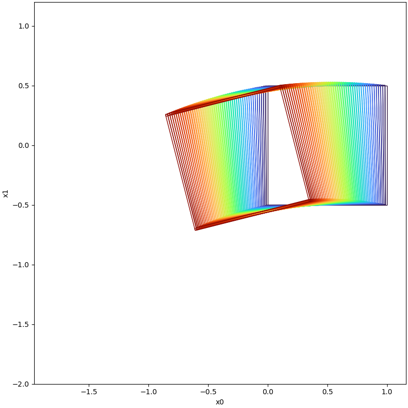 |
 |
| t=1.0 | 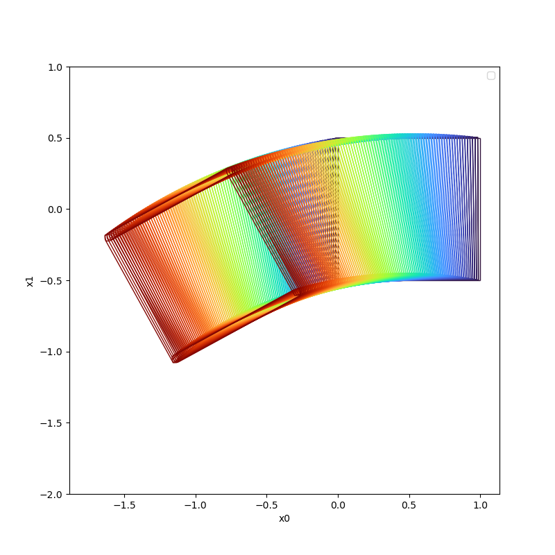 |
 |
| t=1.5 | 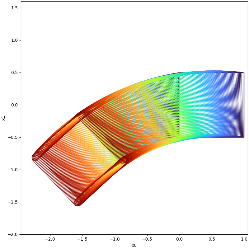 |
Set Explosion Occured! |
Besides the 2D plot and plot_cmp, sets can be shown in 3D with plot3d (projection onto 3 state
dimensions) and plot_tube (2 state dimensions over time). The interactive plotly backend works in
Jupyter and Colab and needs pip install "pybdr[vis]"; backend="matplotlib" draws static figures.
from pybdr.geometry import Geometry, Interval
from pybdr.geometry.operation import boundary
from pybdr.util.visualization import plot3d, plot_tube

# reachable sets of the example above over time
plot_tube(ri_without_bound[1:], [0, 1], step=options.step)

# boxes covering the boundary of a cube, as a static figure
cells = boundary(Interval([0, 0, 0], [1, 1, 1]), 0.25, Geometry.TYPE.INTERVAL)
plot3d(cells, [0, 1, 2], backend="matplotlib", save_file_name="cells.png", show=False)
All plot functions accept show=False and save_file_name and return the figure for further changes.
Two modes of computation are supported by the tool for reachable sets. One mode is to compute the reachable set of evolved states using the entire initial set in a set propagation manner, while the other mode is to compute the reachable set of evolved states based on the boundary of the initial state set.
The computation may be slow for several reasons such as large computational time intervals, small steps, high Taylor expansion orders, or a large number of state variables.
To accelerate the computations, experiments can be performed with a smaller computational time horizon, a smaller order of expansion (such as 2), and a larger time step. Then gradually increase the computational time horizon and order of expansion based on the results of this setting to achieve the desired set of reachable states at an acceptable time consumption.
reach_parallel computes the cells of the boundary in worker processes. On macOS and Windows these
processes import the main script again, so the script must put its computations under
if __name__ == "__main__": as in the examples above. Notebooks (Jupyter, Colab) need no guard, and
dynamics defined in a notebook work with reach_parallel as well.
To enhance the precision of the reachable set computation, one can split the boundaries of initial sets or increase the order of the Taylor expansion while reducing the step size.
Feel free to contact dingjianqiang0x@gmail.com if you find any issues or bugs in this code, or you struggle to run it in any way.
This project is licensed under the GNU GPLv3 License - see the LICENSE file for details.
@inproceedings{ding2024pybdr,
  title={PyBDR: Set-Boundary Based Reachability Analysis Toolkit in Python},
  author={Ding, Jianqiang and Wu, Taoran and Liang, Zhen and Xue, Bai},
  booktitle={International Symposium on Formal Methods},
  pages={140--157},
  year={2024},
  organization={Springer}
}
When developing this tool, we drew upon models used in other tools for calculating reachable sets, including Flow*, CORA, and various others.